Syntax
VLOOKUP(search_value, lookup_table, column_num, [match_type])
- search_value—The value to search for, which must be in the first column of lookup_table.
- lookup_table—The cell range in which to search, containing both the search_value (in the leftmost column) and the return value.
- column_num—A number representing the column position (in lookup_table) of the value to return, with the leftmost column of lookup_table at position 1.
- match_type—[optional]The default is true. Specifies whether to find an exact match (false) or an approximate match (true).
Sample usage
VLOOKUP("Task E", [Task Name]1:Done5, 2, false)
Usage notes
Use a VLOOKUP formula to automatically bring in associated content based on criteria in your sheet. For example, bring in someone's role using their name as the criteria.
- You can use VLOOKUP to reference a cell from another sheet and look up a value from a table in another sheet.
- If VLOOKUP doesn't find a result, you receive a #NO MATCH error message.
- You also receive a #NO MATCH error if there isn't a number within the range that's greater than or equal to the search_value.
- If lookup_table isn't sorted in ascending order by the first column, then VLOOKUP returns incorrect results.
- The search_value must be in the leftmost column (position 1) of lookup_table.
- To look up text strings, you must enclose the lookup value in quotation marks (for example, “Task E”).
- With the match_type argument:
- Set match_type to false if your lookup_table isn't sorted.
- True (the default value) assumes that the range is sorted ascending and returns the nearest match that's less than or equal to ( <= ) search_value.
- False returns the first exact match.
You can insert the column number into a formula to indicate which column you're retrieving the value from.
For example, the formula =VLOOKUP([Inventory Item]3, [Inventory Item]1:[Number of Items in Stock]4, 3, false) returns the value 4. The formula is written to retrieve a value from the third column (Number of Items in Stock) in the table below.
Brandfolder Image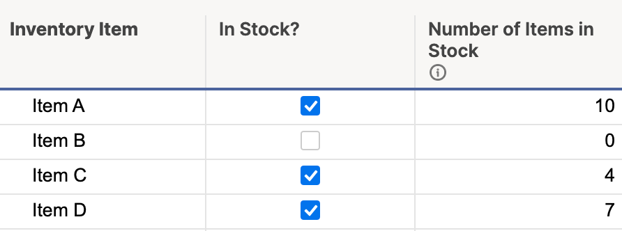
Examples
This example references the following sheet information:
| Clothing Item | Units Sold | Price Per Unit | In Stock? | Status | Assigned To | |
|---|---|---|---|---|---|---|
| 1 | Clothing Item T-Shirt | Units Sold 78 | Price Per Unit $15.00 | In Stock? true | Status Green | Assigned To sally@domain.com |
| 2 | Clothing Item Pants | Units Sold 42 | Price Per Unit $35.50 | In Stock? false | Status Red | Assigned To tim@domain.com |
| 3 | Clothing Item Jacket | Units Sold 217 | Price Per Unit $200.00 | In Stock? true | Status Yellow | Assigned To corey@domain.com |
Based on the table above, here are some examples of using VLOOKUP in a sheet:
| Formula | Description | Result |
|---|---|---|
| Formula IF([In Stock?]1 = 1 (true), VLOOKUP("T-Shirt", [Clothing Item]1:Status3, 5)) | Description Return the status color. If the In Stock column equals 1 (true) look up the value “T-Shirt” in the Clothing Item column and produce the value of the Status column. | Result Green |
| Formula IF([In Stock?]2 = 0 (false), VLOOKUP([Row #]1, [Row #]1:[In Stock?]3, 2)) | Description Return item out of stock. If the In Stock column equals 0 (false) look up the value of Row 2 and produce the value of the Clothing Item, column 2. | Result Pants |
| Formula VLOOKUP("Jacket", [Clothing Item]1:[Price Per Unit]3, 3, false) * [Units Sold]3 | Description Return total revenue. Look up the value “Jacket” in the Clothing Item column. If found, produce the value in the Price Per Unit column ($200). Then multiply this by the Units Sold column value (217). | Result 43400 |
| Formula VLOOKUP([Clothing Item]1, {Range on Reference Sheet}, 2, false) | Description Return the assigned to contact email. Look up the value in the Clothing Item column row 1 on the reference sheet. If found, produce the value in the Assigned To column. | Result sally@domain.com |
Still need help?
Use the Formula Handbook template to find more support, resources, view 100+ formulas, a glossary of every function that you can practice working with in real time, and examples of commonly used and advanced formulas.
Find examples of how other Smartsheet customers use this function or ask about your specific use case in the Smartsheet online Community.

