Syntax
MATCH(search_value, range, [search_type])
- search_value—The value to search for.
- range—The cell range (lookup table) to be searched.
- search_type—[optional][optional] The default is 1. Defines approximate (1, -1) or exact match required (0). In addition, defines whether the range is sorted ascending (1), not sorted (0), or sorted descending (-1).
Sample usage
MATCH("Task A", [Task Name]:[Task Name], 0)
Usage notes
Smartsheet calculates the relative position of a search value by counting cells from left to right (across columns) and top to bottom (across rows). In a lookup table of two columns, the cell in the top row of the leftmost column is the first position, 1.
For the optional search_type argument:
- 1: (The default value) Finds the largest value less than or equal to search_value (requires that the range be sorted in ascending order)
- 0: Finds the first exact match (no sort order is required)
- -1: Finds the smallest value greater than or equal to search_value (requires that the range be sorted in descending order)
Examples
This example references the following sheet information:
| Row # | Clothing Item | Transaction Total | Units Sold | Clothing ID | Price per Unit | Order Date |
|---|---|---|---|---|---|---|
| 1 | T-shirt | $1,170.00 | 78 | A0012 | $15.00 | 02/12/25 |
| 2 | Pants | $1,491.00 | 42 | A0013 | $35.50 | 02/15/25 |
| 3 | Jacket | $900.00 | 45 | A0014 | $20.00 | 02/20/25 |
Based on the table above, here are some examples of using INDEX in a sheet:
| Formula | Description | Result |
|---|---|---|
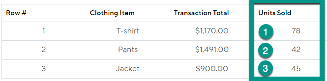
| =MATCH("Pants", [Clothing Item]:[Clothing Item], 0) | Returns the row position for Pants in the Clothing Item column. Requires an exact match. | 2 |
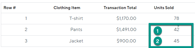
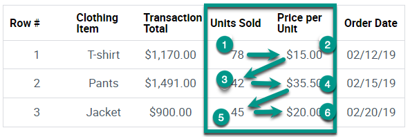
=MATCH(“Pants”, [Clothing Item]:[Clothing ID], 0) | Returns the position of the value Pants from the two-column table, where T-shirt would be 1st position, and A0014 is 6th position. | 3 |
=MATCH(DATE(2025, 2, 12), [Order Date]:[Order Date]) |
This is using the default search_value of 1 (approximate match allowed, ascending sort order). | 1 |
| =MATCH([Clothing ID]@row, [Clothing ID]:[Clothing ID], 0) | Gives the relative position for the Clothing ID on the current row within the sheet. Applying this formula with a unique search_value and a single-column range produces a value equivalent to the Row Number. | |
| =INDEX([Order Date]:[Order Date], MATCH("Jacket", [Clothing Item]:[Clothing Item], 0)) | Returns the value in the Order Date column for the row that contains the value Jacket in the Clothing Item column | 2/20/2025 |
Still need help?
Use the Formula Handbook template to find more support resources and view 100+ formulas, including a glossary of every function that you can practice working with in real-time and examples of commonly used and advanced formulas.
Learn more about formula combinations for cross sheet references.
Find examples of how other Smartsheet customers use this function, or ask about your specific use case in the Smartsheet online Community.