Syntax
INDEX(range, row_index, [column_index])
- range—The column, group of columns, and rows or cross-sheet reference that contains the value you want to return.
- row_index—The position of the row you want to retrieve, counting from the top of the defined range.
- column_index—[optional](Optional) The position of the column you want to retrieve, counting from the left of the defined range. Required when the range covers more than one column.
Sample usage
INDEX([Task Name]:[Task Name], 5)
INDEX(CHILDREN([Task Name]@row), 1)
Usage notes
- The range can be a function that returns multiple values, for example: COLLECT, ANCESTORS, or CHILDREN.
- You can use the MATCH function as the row_index value for INDEX to return an item from a range based on the relative position of a value in another range.
- You can use the COLLECT function as the range value for INDEX to return an item from a list of collected values that meet the specified criteria.
Understand row_index
A frequent source of confusion is row_index. Remember this crucial rule:
row_index and column_index always refer to the position within the range you defined, not the entire sheet.
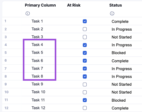
If your range is [Task Name]4:[Task Name]8 (Row 4 to row 8 in your sheet for a total of 11 rows):
- row_index: 1 refers to row 4 of the sheet.
- row_index: 5 refers to row 8 of the sheet.
The row_index must start at 1. Using 0 or leaving the argument blank results in an error.
Examples
Example 1: Simple positional lookup
Use the basic INDEX function when you know the exact numerical position of the value you want.
In your sheet, you have a specific value in one cell that needs to be referenced by all rows in the sheet as a column formula.
You can't simply select the cell, since specific references aren't supported by column formulas. Instead, you can use INDEX to target the specific column and row that your desired value is in.
Scenario: You want to quickly grab the Item Price from the 5th row of the Discount column.
Sheet 1 - Discount values ranked from highest to lowest
| Current coupon codes | Discount |
| SUMMER25 | 25% |
| BACKTOSCHOOL | 15% |
| NEWCUSTOMER | 15% |
| THANKYOU10 | 10% |
Sheet 2
| Item name | Item price | Maximum discount | Lowest item price |
| T-shirt | $15.00 | 25% | $11.25 |
| Pants | $35.00 | 25% | $26.25 |
| Jacket | $200.00 | 25% | $150.00 |
| Hat | $25.00 | 25% | $18.75 |
| Gloves | $45.00 | 25% | $33.75 |
| Shoes | $80.00 | 25% | $60.00 |
Formula:
=INDEX({Discount Codes}, 1)
Result: 0.25
This formula is best for cross-sheet data lookups where the value you need is always in the same row on the target sheet. If you want to reference a specific cell within the same sheet using a column formula, consider adding it to the sheet summary (=Discount1) and then refer to the sheet summary in your desired formula ([Discount Reference]#).
Example 2: Advanced positional lookup
Use INDEX with both the row_index and column_index values when you need to look up a value from a table rather than simply within a single column.
Scenario: You have a prioritization matrix that assigns a priority level based on the Impact and Effort scores of each request. Both scores are already captured as numbers in your sheet, so you can feed them directly into INDEX as the row and column indexes.
Priority matrix (in a separate reference sheet or range):
| Impact\Effort | 1 | 2 | 3 | 4 |
| 1 | Highest | High | Medium | Low |
| 2 | High | High | Medium | Low |
| 3 | Medium | Medium | Low | Low |
| 4 | Low | Low | Low | Lowest |
Requests sheet:
| Request | Impact | Effort | Priority |
| Request A | 1 | 2 | ? |
| Request B | 3 | 1 | ? |
| Request C | 2 | 4 | ? |
Formula (in the Priority column):
=INDEX({Priority Table}, [Impact]@row, [Effort]@row)
The range you include in the formula is from the matrix where your data lives; don't include the axis labels.
| Request | Impact | Effort | Priority |
| Request A | 1 | 2 | High |
| Request B | 3 | 1 | Medium |
| Request C | 2 | 4 | Low |
INDEX pulls the value from the matrix at the row position defined by Impact and the column position defined by Effort. For Request A, Impact = 1 and Effort = 2, so INDEX returns the value at row 1, column 2 of the matrix = High.
If your matrix is on the same sheet as your formula, lock the range with absolute references ($[Column1]$1:$[Column4]$4) so it doesn't shift when the formula copies down.
Example 3: INDEX and MATCH
Most of the time, you don't know the exact row number; you know the value in another column and you want to return the corresponding value from the same row (the “Item price” for "Jacket"). This is where the INDEX + MATCH combo comes in.
The MATCH function searches a column for a specific value and returns the numerical position (row_index) of where it found the match. We then pass that number directly into the INDEX function as the row_index value. For more information on how to use the MATCH Function, see the MATCH help content article.
Formula:
=INDEX(Column_to_Return_Value_From, MATCH(Lookup_Value, Column_to_Search_In, 0))
Scenario: Find the Item Price for the item named Jacket.
| Item name | Item price |
| T-Shirt | $15.00 |
| Pants | $35.50 |
| Jacket | $200.00 |
Combined formula:
=INDEX([Item Price]:[Item Price], MATCH("Jacket", [Item Name]:[Item Name], 0))
Result: $200.00
How it works
- MATCH("Jacket", [Item Name]:[Item Name], 0) searches the [Item Name] column for "Jacket" and returns 3.
- INDEX([Item Price]:[Item Price], 3) uses the result 3 to pull the value from the 3rd position of the [Item Price] column.
The search value for MATCH is often defined as a cell reference, such as [Requested Item]@row in the target sheet, to look up different values on each row based on the contents of a specific column in the source sheet.
What if I need to search based on multiple criteria (find a price for "T-Shirt" and "Size Large")?
Combine INDEX with COLLECT instead of MATCH. The COLLECT can filter a range based on multiple conditions to find the value(s) that meet all the conditions that it then passes to INDEX instead of using the entire column. To use INDEX and COLLECT, you most often define the row index as 1, to return the first and often only value found by COLLECT.
Still need help?
If you have an Enterprise plan, you can use AI to help write and troubleshoot formulas.
Use the Formula Handbook template to find more support resources and view 100+ formulas, including a glossary of every function that you can practice working with in real time, and examples of commonly used and advanced formulas.
Find examples of how other Smartsheet customers use this function or ask about your specific use case in the Smartsheet online Community.