Learn how to create and modify chart widgets, using AI or manually. Customize chart types, titles, axes, series data, legends, and widget behavior.
USM Content
Create charts directly from your sheets or reports. You have three ways to create a chart:
- Chart > Build with AI: Create a chart using a prompt. Just select your source sheet and select one of the suggested prompts or enter your own, without needing helper sheets or intermediate assets first. Only sheets are supported as source data.
- Chart > Build manually: Manually select your source sheet or report and edit the display and widget behavior from the editing panel. You can then build and edit the generated chart manually, without needing helper sheets or intermediate assets first.
Only charts built with AI or manually are filterable.
- Chart > Build legacy chart: Manually select your source sheet and data. Data is visualized as displayed in the sheet, this means you might need to manually prepare your data to visualize it as desired. Charts built with the legacy experience are not filterable.
For a better filter experience, use your main sheet or report as a source. Metrics or metadata sheet have limited data for filters to apply correctly.
Regardless of the widget experience you select, ensure you are using supported column types: Text/Number, Dropdown list, Auto-Number/System-generated column and Symbols. The widgets skip any cells containing text, symbols, or non-integer values.
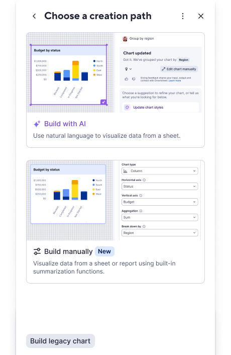
Choose a chart creation path
Build with AI and Build manually add raw data for you inside the chart widget, without needing metric sheets, use source data directly from primary sheets.
Legacy charts are available if you prefer to create your own metrics sheet or prepare data ahead.
See the comparison below to select your preferred approach.
| Build with AI and Build manually | Legacy chart | |
|---|---|---|
Data source | Sheets (Build with AI); sheets or reports (Build manually). | A cell range from a sheet or report. |
Data prep | None. Point at your raw data and choose how to summarize it. | Data must already be laid out as a summary table (labels in the top row and left column). |
Multi select columns | Not supported. Group By is available. | Supported. |
Group by | Add a second dimension for stacked or grouped charts. | Not available. Use separate columns in your range. |
Switch rows columns | Not supported. | Supported. |
Use column names as category labels | Not supported. | Supported. |
Aggregation | Count, Sum, Average, Min, Max, Median. | Not available. Summarize your data in the sheet first. |
Chart types
You can choose from the following chart types:
- Line
- Smooth line
- Stepped line
- Bar
- Stacked bar
- Column
- Stacked column
- Pie
- Donut
- Scatter (Only legacy charts)
Pie and donut charts don't display zero values
Create a chart > Build with AI
AI tools are only available for Trial and Enterprise plans.
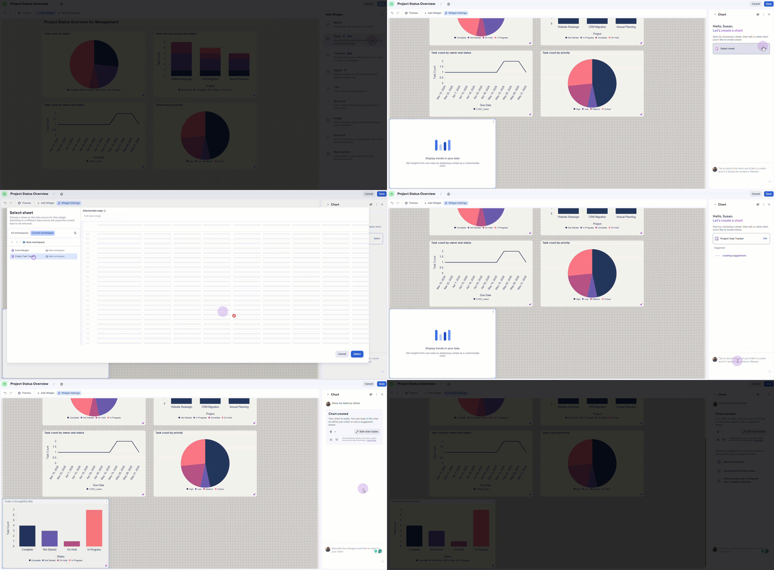
- From the Widgets panel, select the Chart widget.
- Select Build with AI.
- Select a sheet to use as your data source.
- Describe the chart you'd like to create in your own words, or pick from the suggested prompts
- Chart previews are displayed.
AI outputs provide a short explanation of how it generated the chart.
Create a Chart > Build manually
- From the Widgets panel, select the Chart widget.
- Select Build manually.
- Select a sheet or report to use as your data source and the data you want to visualize.
- Edit as desired using the fields in each section of the panel. Refer to the Edit a Chart section below for details on the availablie fields.
- Select Save to add it to your dashboard.
Create a chart > Legacy chart
- From the Widgets panel, select the Chart widget.
- Select Legacy chart.
- Select Add Data in the Data & Chart Type section.
- On the left side of the form, select the sheet or report that contains the table you want to chart. Then select the range of cells on the right side.
- Once you have your data, select OK.
If you need to change your data range later, edit the widget and select Edit Data to reselect the data range. Once you've selected your data, select a chart type and formatting.
- Select your desired chart type.
- Set up your chart (refer to the Edit a chart section below)
- Select Done.
Edit your chart
How you edit your chart depends on how you created it.
Edit a chart built with AI:
- Select an existing chart.
- Select Edit with AI to use prompts to refine it or.
Edit a chart built manually:
- Select an existing chart.
- Use the displayed fields to manually edit your chart. In addition to the editable options explained in the table below, you have the following:
- Aggregation: select how to summarize your data: Count, Sum, Average, Min, Max, or Median.
- Break down by: add a second dimension to create a stacked or grouped chart.
- Display style: change the chart type.
Edit a chart built with the legacy experience
- Select an existing chart.
- Use the displayed fields to manually edit your chart. Refer to the table below for details on the available edit options.
Edit options available in charts
| To do this | Follow these steps |
|---|---|
Chart only certain columns from the selected range | Select Columns Included and select only the columns you want to display. |
Ignore the text labels in the cells of your table. | Toggle on Use column names as category labels. |
Use the top row of your sheet as labels | Toggle off Use first column as series labels. |
Switch how columns and rows are plotted on your chart. | Toggle on/off Switch rows/columns. |
Change the chart type. | Use the dropdown to select the Chart type you want to use |
Add a title to your chart. | Expand the Title section and enter your title.
|
Configure the horizontal/vertical axis of your chart. | Expand the Horizontal Axis or Vertical Axis section and enter the Axis title. Use the Title styling and Axis labels styling options to format the title and labels. |
Add gridlines to your chart (except pie charts). | Expand the Horizontal Axis or Vertical Axis sections and toggle on or off Show tick mark lines. |
Edit series data. | Expand the Series section. Select which series to edit in the Apply to field. Select the desired Color. You can Toggle on or off the Always show value label and Fill line options. |
Change the colors of the data or add labels to the data plotted in your chart. | Expand the Series section, select the series to edit the color in the Apply to field. By default, white text appears on a dark background, and black text appears on light backgrounds. |
Label slices of a pie chart with a percentage of the whole or actual values. | Expand the Pie Chart or Donut Chart section, and use the dropdown under Value Labels to select one of the following:
You can change the colors for each section of the pie chart and toggle on/off the option to display it as a semicircle. |
Add or move a legend on your chart. | Expand the Legend section and select the Legend position. Use the Legend styling options to format the it. |
Select how viewers see the widget | Expand the Viewer mode section. Select from:
Hover over What’s the difference? For details. |
Edit the widget's interaction (what happens when you select the widget). | Select Widget Behavior and choose one of the interaction options:
|
Pie and Donut charts: display as a half-pie or half-donut | Expand the Pie Chart & Series section and enable the Display as semicircle toggle. |
Existing charts on dashboards created with the analyze data AI tool aren’t editable yet. We are working to make it available soon.
Use the Analyze data AI tool
Smartsheet's analyze data AI tool offers an intelligent way to generate charts directly from your sheet. Instead of manually selecting data ranges and chart types, you can simply ask a question to create the chart widget you want.
Refer to Use analyze data to generate charts and metrics for more details.
Frequently Asked Questions
I want to use the data in the top row of my table as labels, but the chart is using my column names instead. How do I fix this?
When values are in the top row of your data, the charts widget assumes these values are meant to be plotted and uses the column names as labels instead. To force the top row of your table to be used as labels, uncheck Use column names as category labels.
Can a chart be created from data in more than one sheet?
Currently, charts can only be created against data in a single sheet or report. If your source data is on multiple sheets, create a report to collect the information, or use cell links or a formula that references data from another sheet to collect your data into one sheet. More information on these options can be found in the following help center articles:
My custom color configuration doesn’t display on an existing chart. How do I save a custom color configuration to a series in a chart?
When a chart uses a row-based grouping and summary report, and only one column is selected under Columns Included in the chart widget Editor, you can't save a custom color configuration for the charted series.
If you change the series colors from the default, the system reverts them to the default colors when you save.
To fix this:
- Edit the chart widget. For more information on how to edit a chart, see Customize the format of your chart.
- Under Columns Included, select the primary column to name the series.
- Select Series, then select each value to update color choices. Once you save, the custom color configuration displays on the chart and persists.
My chart labels disappear. What should I do?
Smartsheet occasionally hides labels to highlight the chart and improve legibility. To showcase the label, either lower the font size or resize the widget.